Zero-K: How effective is wind, really?
This post expands upon my forum post here,
which did a deep dive into the energy efficiency of wind power in Zero-K. Zero-K is a free and open source
RTS game, following the Total Annihilation style. Conventional wisdom
was that Wind was “worth it”, when the minimum was at least
+0.2e/s (energy per second).
A diminishing returns economy
One of the more interesting features in Zero-K compared to its peers is the diminishing “overdrive” economy, rather than the exponential metal-maker economy of most TA-likes. The Zero-K wiki has a detailed guide on the economy, but the short version is: Excess energy is converted to metal at a rate which reduces in effectiveness the more energy is converted. This means that in the early game, when energy can be converted to metal at a very high rate, the choice of economy matters a lot.
The diminishing returns of the overdrive economy are implemented as a square root. Specifically, where \(E\) is the amount of overdrive energy allocated to that specific mex, a mex produces metal at its face value multiplied by:
\[ 1 + E^{0.5} / 4 \]
So if your mexes produce a total of +100m/s (metal per
second), and there is 100e/s excess energy for overdrive,
the amount of metal you get depends on how that is divided:
- If you have four mexes at
+25m/s, each mex receives+25e/sfor overdrive, gaining a multiplier of 225% taking them to56.25m/seach, for a combined total of225m/s. - If you have fifty mexes at
+2m/s, each mex receives+2e/sfor overdrive, gaining a multiplier of 135% taking them to2.7m/seach, for a combined total of135m/s.
Basic energy structure efficiency
In the early game, you have two options for cheap energy generation:
Wind and Solar. Wind is cheap, random, and fragile, but is generally
more cost effective, producing between a map and height based minimum,
generally up to +1.0e/s, and a maximum of
+2.5e/s. Solars have a slightly higher fixed cost, but fold
up, turning themselves off, and becoming extremely durable when raided.
Solars produce a consistent +2e/s.
In-game, Zero-K does a pretty fair job of estimating how long energy structures will take to pay for themselves. If a smaller energy structure would pay for itself in the time it would take for a larger energy structure to complete, you’d be better off building the smaller energy structure first, since you’d finish the larger structure in the same time, plus you also have the smaller structure.
Expressed in terms of metal-seconds per energy output, the structures have the following cost efficiency, least to most efficient, picking specific lower-bound examples for wind generators:
| Structure | Cost (m) | Energy output (e/s) | Cost efficiency (\(mse^{-1}\)) |
|---|---|---|---|
| Solar Collector | 70 | 2 | 35 |
| Tidal | 35 | 1.2 | \(29.166\dots\) |
| Fusion Reactor | 1000 | 35 | \(28.5714\dots\) |
| Wind (0.0 lower bound) | 35 | 1.25 | 28 |
| Wind (0.5 lower bound) | 35 | 1.5 | \(23.3\dots\) |
| Geothermal Generator | 500 | 25 | 20 |
| Wind (1.0 lower bound) | 35 | 1.75 | 20 |
| Singularity Reactor | 4000 | 225 | \(17.78\dots\) |
| Advanced Geothermal Generator | 1500 | 100 | 15 |
- Solars are robust but ineffective.
- Fusion Reactors are compact, and so more easily defended, especially if you can give them the safety of putting them underwater.
- Singularity Reactors are extremely effective, and an extremely attractive target to match.
- Upgraded Geothermal Generators are so obscenely effective that, even though they’re a nice shiny target, they’ll almost always pay for themselves even if they’ve only survived for a short amount of time.
Wind efficiency is a very deep rabbit hole. Even at ground level, Wind always beats Solar, and barely requires anything (either in terms of height, or other factors like wind grids finishing incrementally) to beat basic Fusion, assuming that all your stable energy needs are met and you’re only concerned with overdrive output.
Wind efficiency
The above table is correct for metal seconds per energy, but when
thinking about overdrive you want to be thinking about the overdrive
multiplier. Overdrive has diminishing returns over the squareroot
function, so Wind is less effective because running at
+.5e/s below average, even if you run at
+.5e/s above average for the same amount of time later, is
worse than just running at average.
Interactive Desmos graph where you can experiment with the parameters here. This interactive graph exposes two simplified equations for wind efficiency.
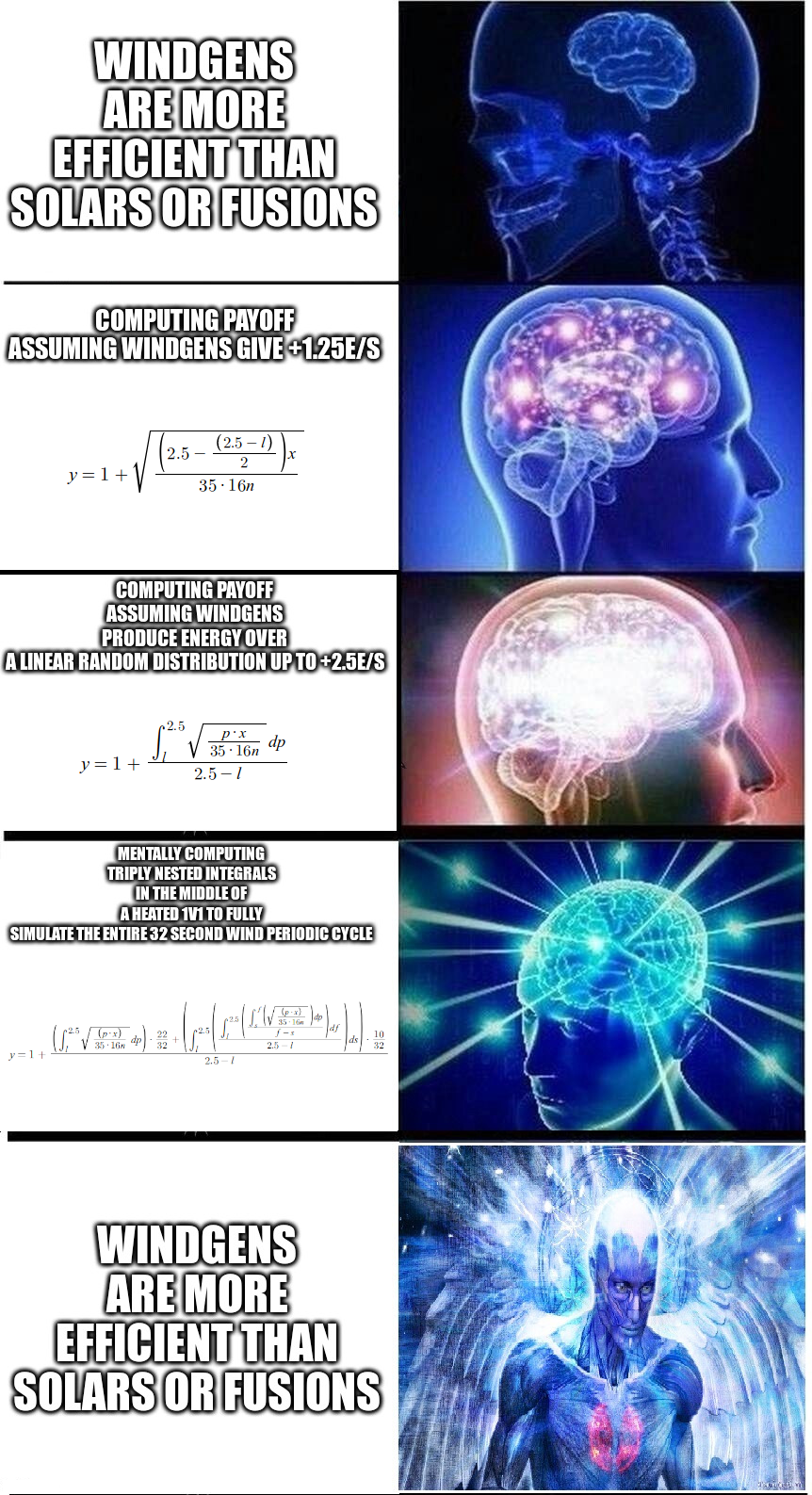
This model simply assumes that a Wind Generator will always produce its mean energy value as output:
\[ y=1+\sqrt{\frac{\left(2.5-\frac{\left(2.5-l\right)}{2}\right)x}{35\cdot16n}} \]
This model assumes that a Wind Generator will produce a linearly
random amount of energy, between its lower bound and
+2.5e/s. This means its average output is slightly
lower:
\[ y=1+\frac{\int_{l}^{2.5}\sqrt{\frac{p\cdot x}{35\cdot16n}}dp}{2.5-l} \]
While ground level wind still produces more raw energy than Fusion on
average, they only start producing more metal (from energy via
overdrive) than Fusions on average once they reach a lower bound of
+0.2e/s, since the diminishing returns of overdrive makes
Fusion stability better, even if all of your
stable energy needs are already met! You still probably don’t
want to be going mostly wind until you reach a lower bound of about
+0.4e/s, though.
Going even further beyond
However, this doesn’t completely model the wind periodic cycle. Wind speed is not a truly linear distribution: Every 10 seconds out of 32, it is moving linearly between two linearly random values, then stays stable for a 22 seconds, then repeats. This means that Wind is more likely to produce values near the middle of its range, and so provides power more stably than the linear model above would predict.
The following formula will fully model wind overdrive efficiency over the wind periodic cycle. However, this is about the point that Desmos starts sobbing uncontrollably and asking what it ever did to deserve this, as it fails to render, and only comes back to render the other functions after about a minute of busy processing that appears to involve webworkers in ways that I am not interested in tracing:
\[ y=1+\frac{\left(\int_{l}^{2.5}\sqrt{\frac{\left(p\cdot x\right)}{35\cdot16n}}dp\right)\cdot\frac{22}{32}+\left(\int_{l}^{2.5}\left(\frac{\int_{l}^{2.5}\left(\frac{\int_{s}^{f}\left(\sqrt{\frac{\left(p\cdot x\right)}{35\cdot16n}}\right)dp}{f-s}\right)df}{2.5-l}\right)ds\right)\cdot\frac{10}{32}}{2.5-l} \]
Not to be defeated, you can always throw numpy+scipy at the problem to get an idea of how much the divergence is:
import numpy as np
from scipy.integrate import quad


def linear_model(n,l,x):
  return 1 + quad(lambda p:np.sqrt(p*x/(35*16*n)), l, 2.5)[0] / (2.5 - l)

def full_model(n,l,x):
  return 1 + (
    quad(
      lambda p: np.sqrt(p*x/(35*16*n)),
      l,
      2.5
    )[0] * 22/32
    +
    quad(
      lambda s:
        quad(
          lambda f:
            quad(
              lambda p: np.sqrt(p*x/(35*16*n)),
              s,
              f
            )[0] / (f - s) if f != s else 0,
          l,
          2.5
        )[0] / (2.5 - l),
      l,
      2.5
    )[0] * 10/32
) / (2.5 - l)display([full_model(2,0.02,x) - linear_model(2,0.02,x) for x in range(0,10)])
display([full_model(2,0.02,x) - linear_model(2,0.02,x) for x in range(10,20)])[0.0,
0.0002224839773998788,
0.0003146398586824084,
0.00038535355328073173,
0.00044496795545656553,
0.0004974892981144396,
0.0005449722214081465,
0.0005886372758061587,
0.0006292797174807241,
0.0006674519332559026]
[0.0007035561125969814,
0.0007378958760879684,
0.000770707106698687,
0.0008021773897883833,
0.0008324588188410864,
0.0008616767406925963,
0.0008899359110712268,
0.0009173249403600092,
0.0009439195763258912,
0.0009697851756813591]import matplotlib.pyplot as plt
from IPython.display import display
xs = list(range(0, 5000, 50))
deltas = [full_model(2, 0.02, x) - linear_model(2, 0.02, x) for x in xs]
fig, ax = plt.subplots(figsize=(8, 4.5))
ax.plot(xs, deltas, marker="o", linewidth=1.5)
title = "Absolute difference: full_model - linear_model (n=2, l=0.02)"
ax.set_title(title)
ax.set_xlabel("Metal investment")
ax.set_ylabel("Metal overdrive multiplier delta")
ax.grid(True, alpha=0.3)
fig.tight_layout()
display(fig, metadata={"caption": title})
plt.close(fig)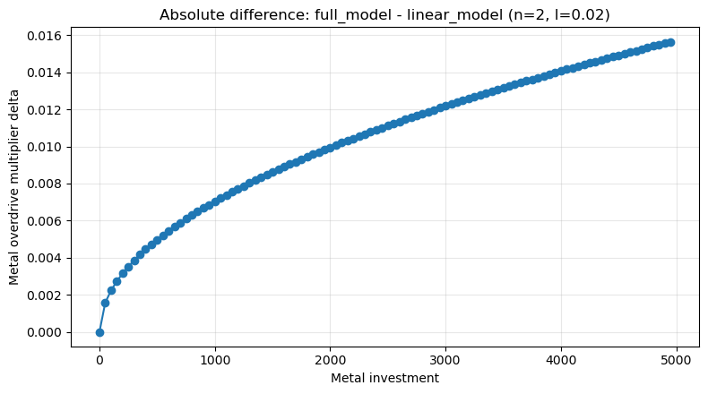
from IPython.display import display

deltas = [full_model(2, 0.02, x) / linear_model(2, 0.02, x) for x in xs]

fig, ax = plt.subplots(figsize=(8, 4.5))
ax.plot(xs, deltas, marker="o", linewidth=1.5)
title = "Relative difference: full_model / linear_model (n=2, l=0.02)"
ax.set_title(title)
ax.set_xlabel("Metal investment")
ax.set_ylabel("Metal overdrive multiplier ratio")
ax.grid(True, alpha=0.3)
fig.tight_layout()

display(fig, metadata={"caption": title})
plt.close(fig)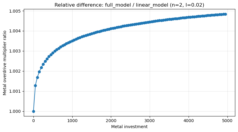
So, you’re fine to just use the linear model for all practical cases.